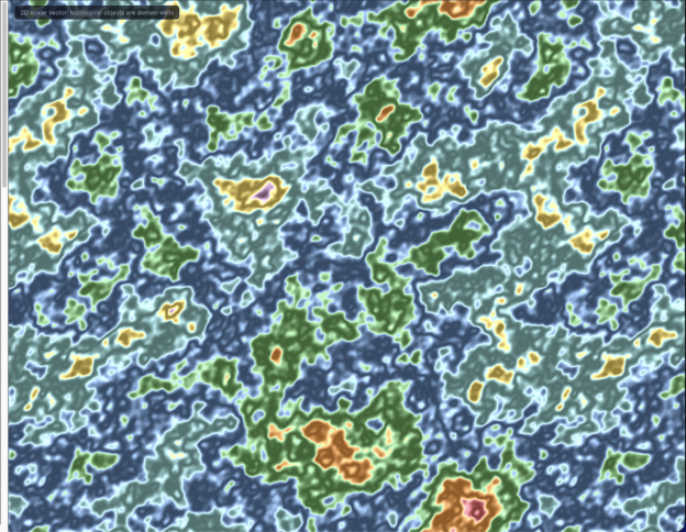
I’ve published a live, interactive visualization of the field at the heart of my physics research program, and you can run it in your browser right now, with nothing to install:
novaspivack.github.io/ugp-physics/visualizations/phimdl_kink_dynamics
This is not an artist’s rendering or a cartoon of the theory. The app integrates the actual field equation — the same equation analyzed in my papers — in real time, on your machine, and lets you poke it: drop particles onto a line with your mouse and watch them collide, paint domains of different vacua onto a plane and watch the walls between them move, and rotate around the three-dimensional structures the theory says are actually there. Every panel is labeled honestly with what is exact, what is a proxy, and what is an illustration, because those distinctions are part of the science.
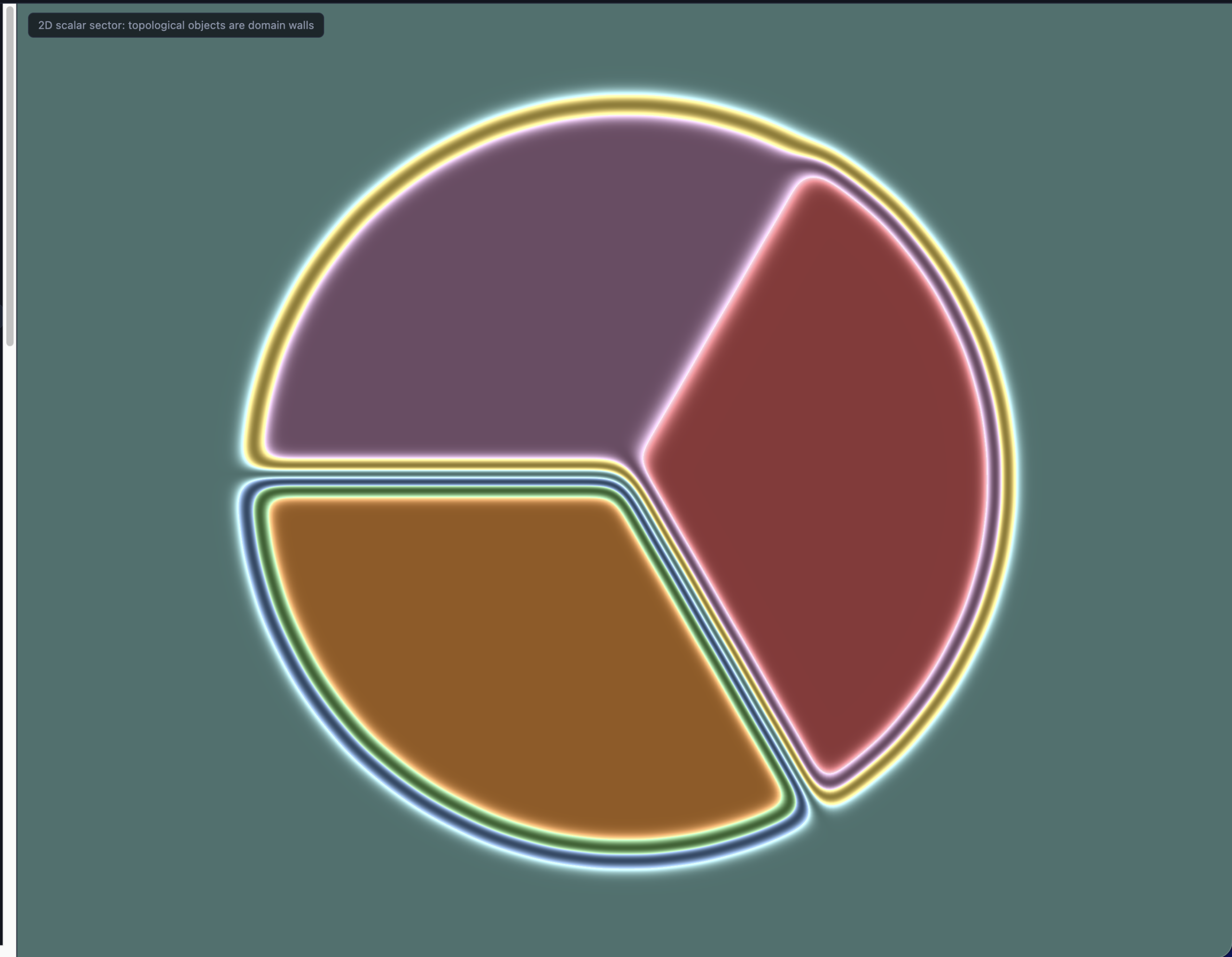
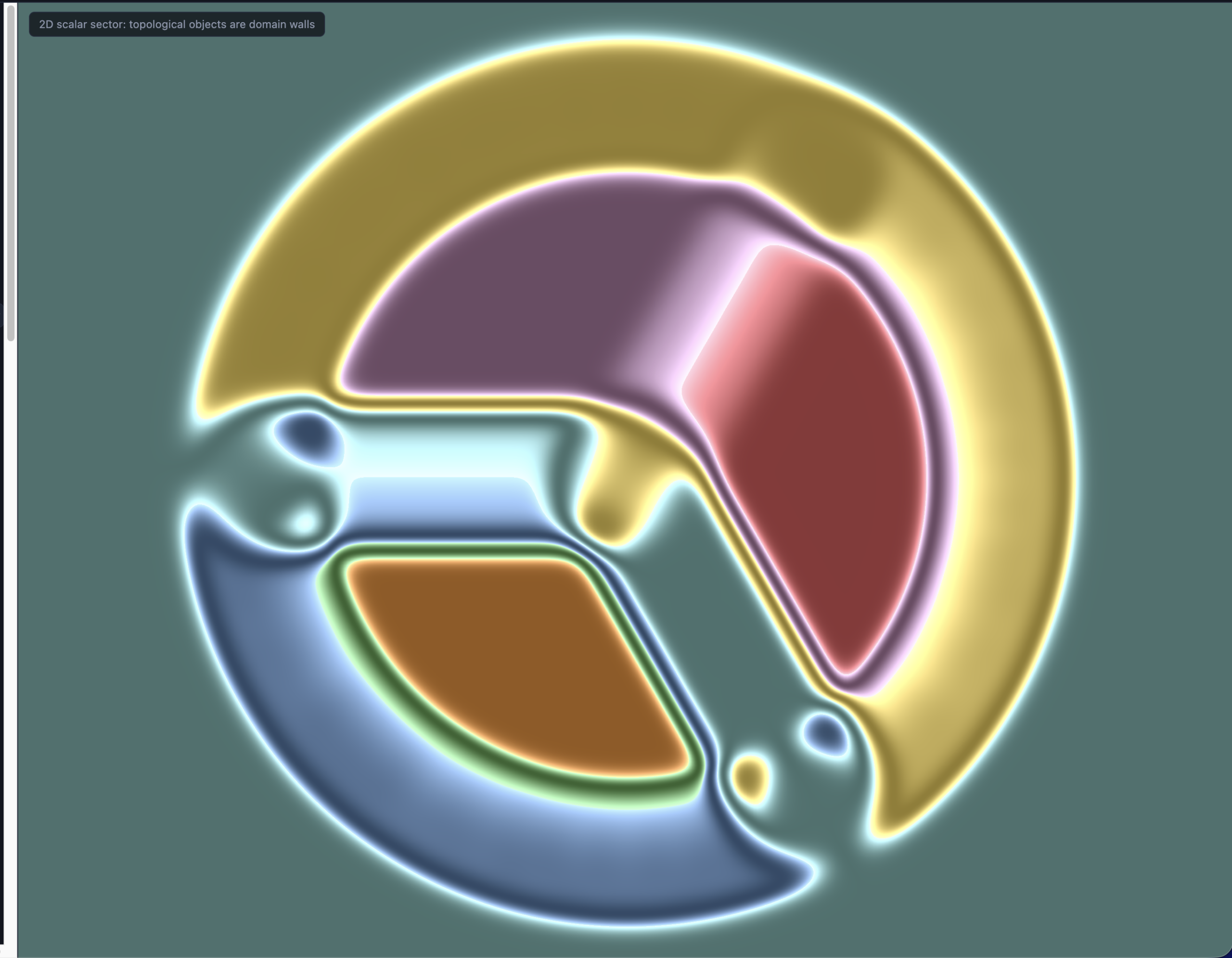
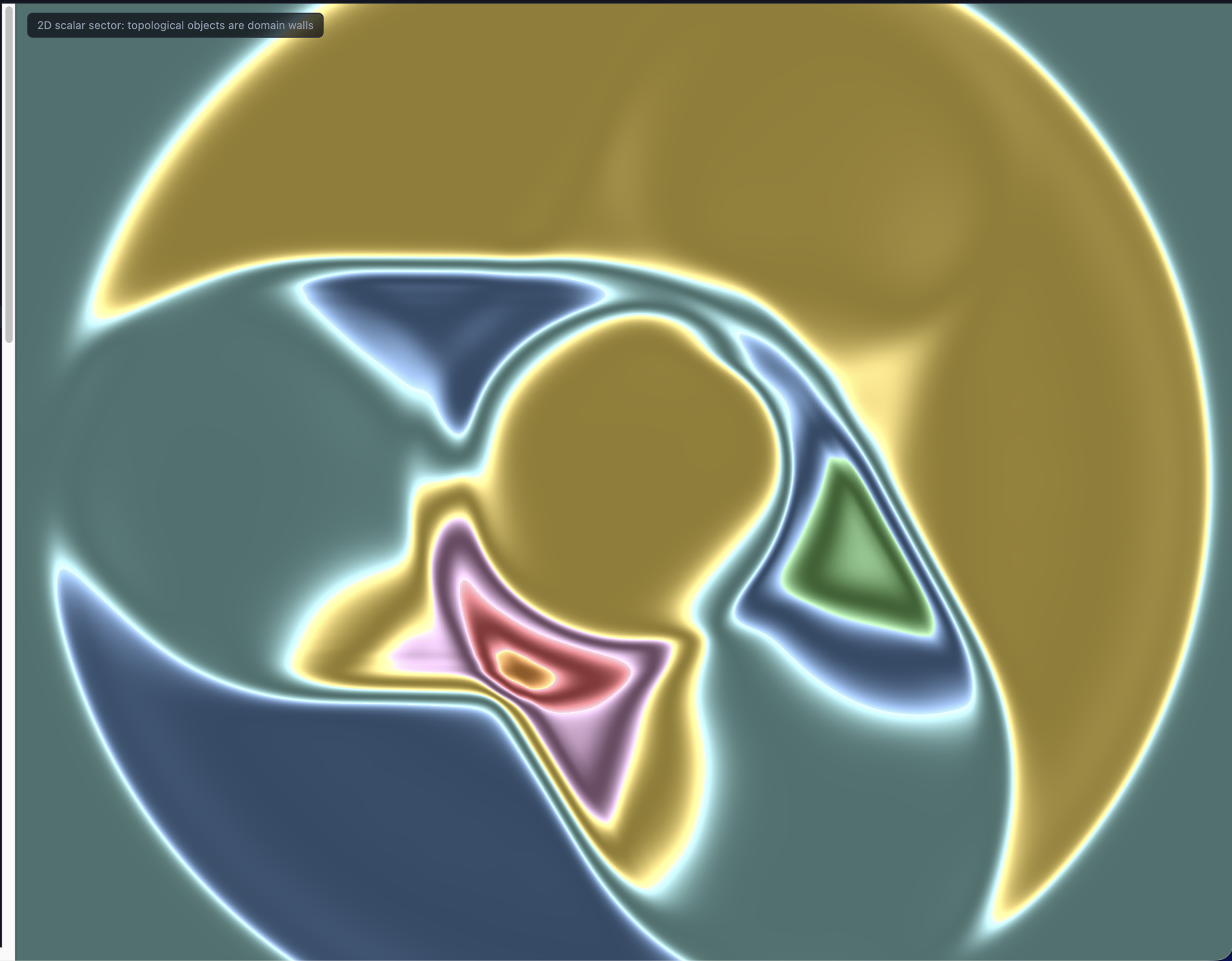
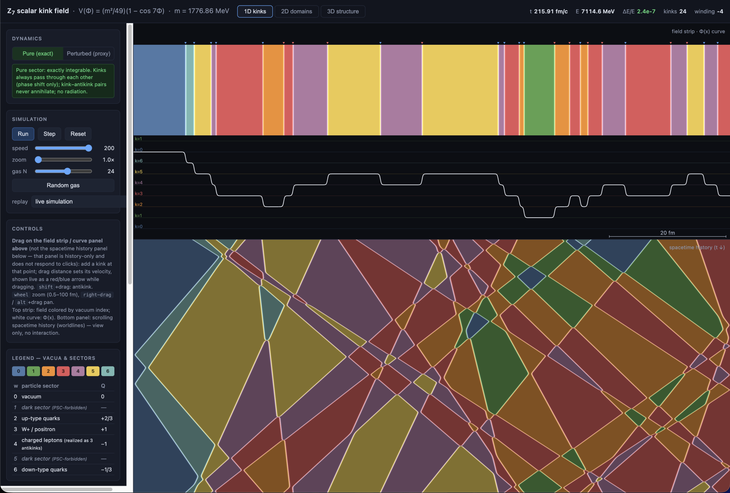
This post explains what you’re looking at.
The field in question
My research program — the Generative Triple Evolution (GTE) framework, built on what I call the Universal Generative Principle — makes an unusually specific claim: the structure of the Standard Model of particle physics can be derived, rather than postulated, from a single small algebraic object. That object is a 19-bit polynomial over the finite field GF(7), and the framework’s statement of the theory fits in two equations: the polynomial (a discrete algebraic certificate that fixes what structures physics must contain) and a continuum field that realizes those structures physically. The framework has zero free dimensionless parameters; a single dimensional anchor, the tau lepton mass, sets the overall energy scale.
The continuum field is called Φ_MDL (the subscript stands for Minimum Description Length, the selection principle that forces its form). It is a scalar field — a single number at every point of space and time — governed by the Lagrangian
L = ½(∂Φ)² − (m²/49)(1 − cos 7Φ)
The important feature is the cosine. Its potential energy landscape has seven degenerate vacua — seven distinct “valleys,” equally spaced, all at exactly zero energy — and an exact Z₇ symmetry that shifts the field from any valley to the next. Empty space means the field is resting in one of the seven valleys. It doesn’t matter which one; they’re perfectly equivalent.
The interesting objects are the transitions. A kink is a region where the field climbs out of one valley and settles permanently into an adjacent one. Once formed, a kink cannot smoothly disappear on its own: undoing it would require rewinding the field everywhere on one side of it, which costs unbounded energy. That robustness is topological — it comes from the global shape of the configuration, not from any local property — and it is the framework’s origin of particle stability.
Nothing in this field is tuned. The mass parameter m is fixed by a self-consistency condition (SCC), derived in the theory papers: the theory’s single dimensionful parameter must equal the mass of the heaviest lepton it generates, the tau, so m = 1776.86 MeV. From that, everything else follows arithmetically: the kink’s spatial width is 1/m ≈ 0.111 femtometers (right at the scale of nuclear physics), and the rest mass of a single elementary kink is (8/49)·m = 290.10 MeV — with the kink-mass result machine-verified in Lean 4, and no adjustable inputs anywhere.
Which kink is which particle
Because there are seven vacua, a field configuration can wind through them by different amounts, and the winding number w — how many valley-steps the field traverses, counted mod 7 — is an exactly conserved charge. The framework’s central identification, derived rather than assigned, is that winding sectors are Standard Model particle classes. Electric charge falls out of a simple formula (Q = w_c/3, using the representative of w centered around zero):
| Winding w | Charge Q | Particle class |
|---|---|---|
| 0 | 0 | Vacuum / photon / neutrino |
| 2 | +2/3 | Up-type quarks (u, c, t) |
| 3 | +1 | W⁺ boson / positron |
| 4 | −1 | Charged leptons (e, μ, τ), W⁻ |
| 6 | −1/3 | Down-type quarks (d, s, b) |
Two sectors are missing from the table: w = 1 and w = 5. Those are excluded by a consistency requirement of the framework (Perfect Self-Containment, PSC); they correspond to dark-sector mirror partners that are not stable states in our branch of the theory. And one subtlety worth knowing: no single stable kink spans more than one valley-step, so the charged-lepton sector w = 4 is physically realized as three elementary antikinks (4 ≡ −3 mod 7), which is both the lower-energy realization and exactly what the charge formula requires: Q = (4−7)/3 = −1.
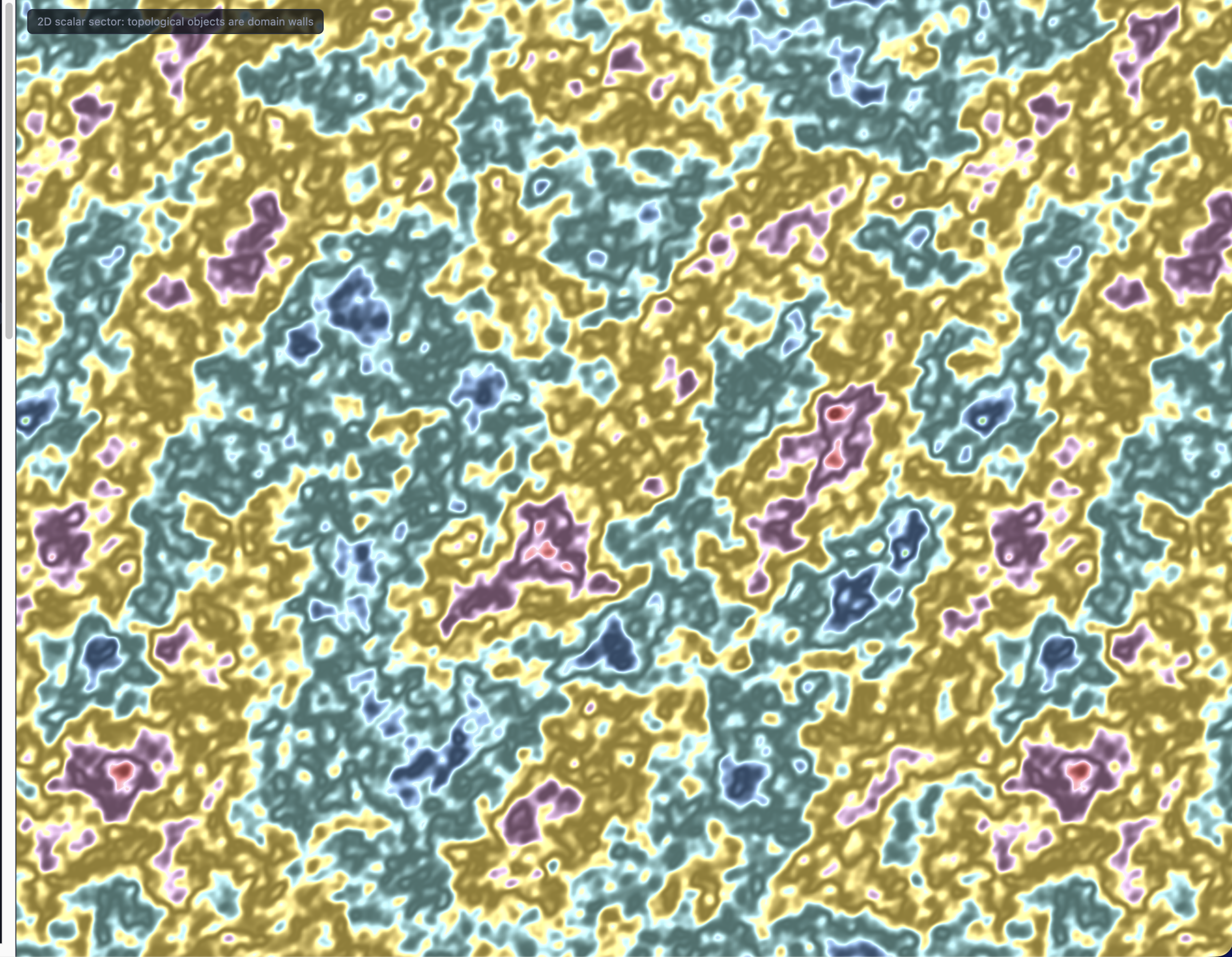
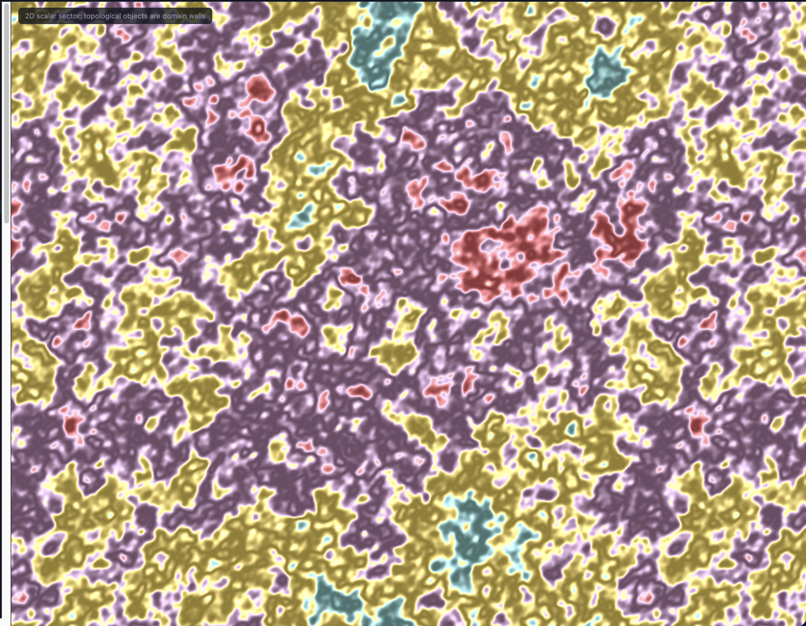
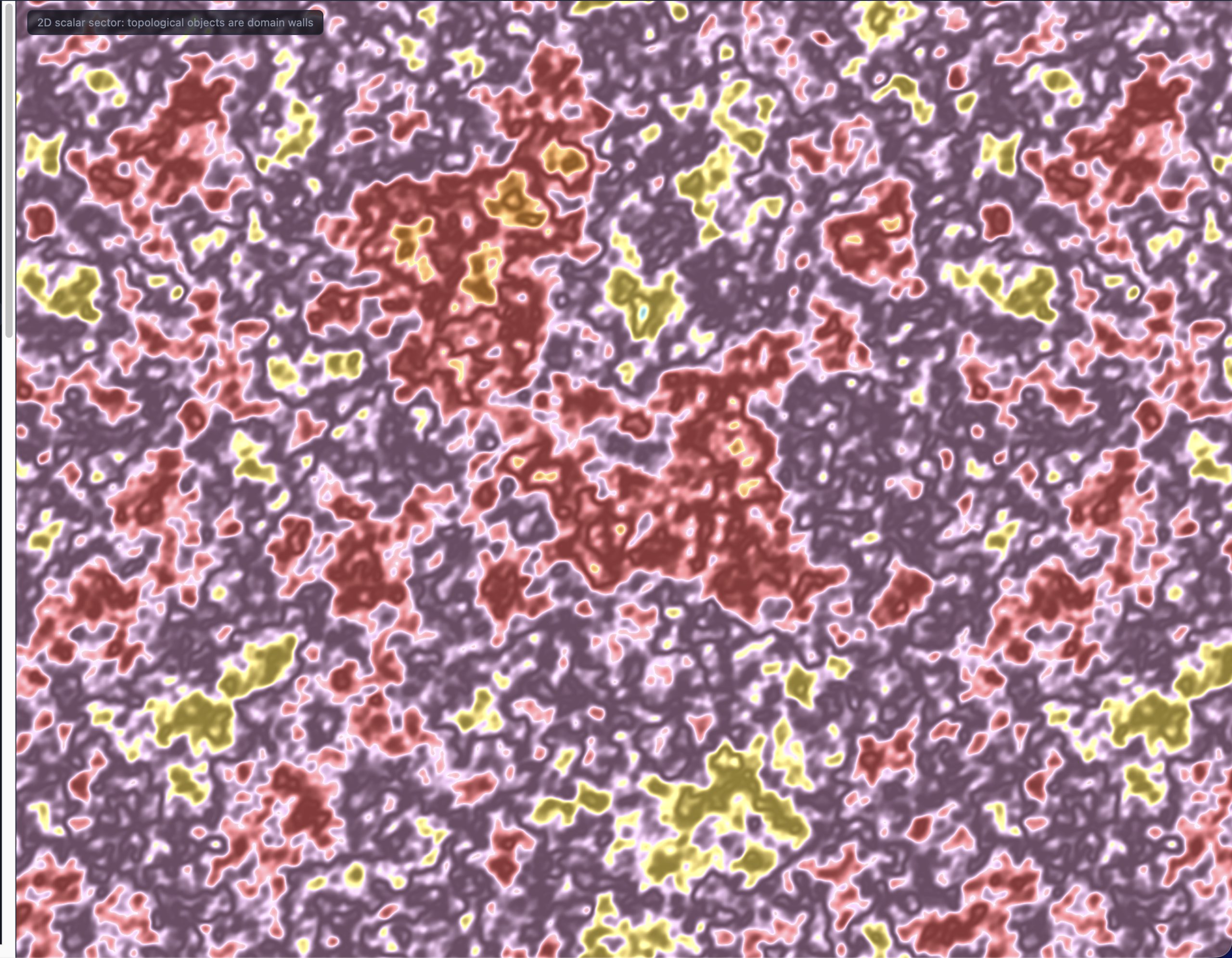
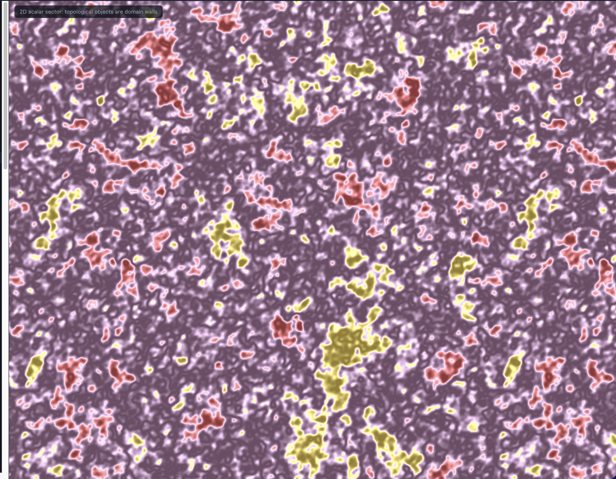
The three generations — why there’s an electron, a muon, and a tau rather than just one charged lepton — do not come from the winding number, which is 4 for all three. They come from the discrete arithmetic level of the framework, where a cascade generates exactly three orbit types. All of this is what the app’s color legend encodes: each of the seven vacua has a hue, and the boundaries between colors are the particles.
So what is a particle? (The part most visualizations get wrong)
Here is where the theory is subtler — and more honest — than the picture you might expect, and the app is built around that honesty.
In one spatial dimension, a kink really is a localized, particle-like lump: a sharp, stable transition at a definite position, carrying definite energy. It is tempting to extrapolate: surely in three dimensions a particle is a little compact ball of field, a “knot” floating in space?
It provably is not. One of the results in the complete-theory monograph is a general no-go theorem: in two or more spatial dimensions, no compact, finite-energy field configuration of this theory can carry winding. The proof of the topological core is almost embarrassingly short once you see it: if a configuration looks the same in every direction far away, its far-field is a single point in the discrete seven-valley vacuum set, and a configuration whose boundary is one point cannot wind anywhere — so its winding is zero. Anything that does wind must therefore look different in different directions at infinity: it must be an extended structure, like a domain wall stretching across space, whose energy grows without bound with its area. The theorem covers every escape route tried — curved walls, pinched walls, string-like defects, time-periodic configurations — and closes them all.
So if particles aren’t compact lumps of field, what are they? The framework’s answer, machine-certified in Lean 4 with zero unproven steps (“zero sorry,” in Lean terminology), is the Fock-space characterization: a particle is a quantized excitation — a state in the quantum theory built on the field — living in one of the topological winding sectors. The sectors are “superselected”: no physical process mixes them, which is why particle identity is an exact quantum number rather than a statistical tendency. The classical extended structure (the wall) is what certifies that the sector exists and fixes its quantum numbers; the particle itself is the normalizable quantum state in that sector.
The slogan I find most useful: the field is everywhere; the topology is what’s quantized. What makes an electron an electron is not a substance sitting at a location — it’s a winding number, w = 4, that the universe’s field carries in that sector and cannot lose except by meeting a positron (w = 3, and 4 + 3 = 7 ≡ 0: the vacuum restored).
Crucially, none of the framework’s particle physics ever depended on the compact-lump picture the no-go theorem rules out: masses come from the discrete cascade arithmetic, charges from the winding formula, statistics from the multiplicative structure of Z₇, stability from superselection. The theorem removes a naive mental image, not a result.
What each mode shows
1D: exact, integrable particle dynamics — live
The 1D mode is the heart of the app, and it is exact in a strong sense. The pure Φ_MDL potential in one spatial dimension is an integrable field theory (it maps exactly onto the sine-Gordon model under a rescaling), which means its multi-kink dynamics are solvable in closed form.
Drag anywhere on the field strip to place a kink — the drag distance sets its velocity — or shift-drag for an antikink, or spawn a random gas of up to 40 of them. Then watch the worldlines in the scrolling spacetime panel. In Pure dynamics you will see something remarkable: kinks and antikinks never annihilate. They pass through each other elastically, every time, at every speed, emerging with only a characteristic spatial phase shift. That’s not a numerical accident; it’s integrability, and the app lets you verify it against theory directly. Open the Advanced panel and switch on “Show exact solution”: the app overlays the exact closed-form N-soliton solution (via the Hirota construction) for whatever kinks you’ve placed, on top of the live simulation, and reports the discrepancy between them. The residual is tiny but not zero — it grows slowly from ordinary discretization drift in the integrator — and that small, stable, honestly-reported residual is exactly what a correct numerical simulation of an exact solution should show.
Real particles, of course, do annihilate. In this framework, annihilation requires breaking the integrability, which in the full theory is done by the gauge-sector coupling (whose derived effect is computable and turns out to be strongly suppressed at ordinary collision speeds). The app’s Perturbed mode illustrates the mechanism with a clearly-labeled proxy: a small symmetry-preserving perturbation to the potential. With it switched on, slow kink–antikink pairs no longer pass through each other — they capture into an oscillating bound state that decays by radiating its energy away until the pair has genuinely annihilated. The app labels this mode as a proxy (provisional, not the derived first-principles coupling), and that label matters: the qualitative capture-and-radiate mechanism is the physically correct picture, while its numerical rates here are illustrative. Two bundled replay runs — a 24-kink pure gas and a 12-kink perturbed gas containing three annihilation events — let you watch both regimes without setting anything up.
2D: domain walls, coarsening, and a live measurement
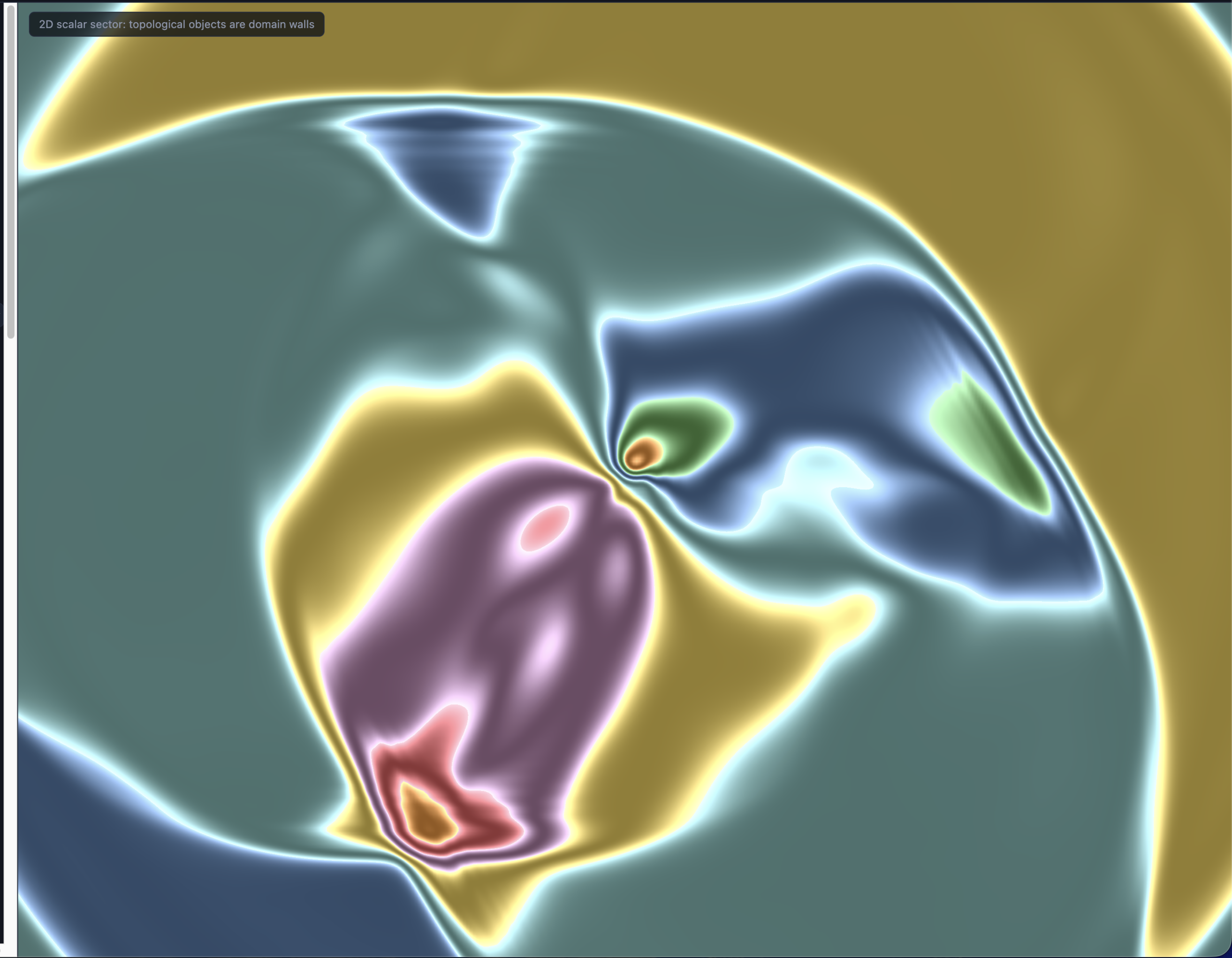
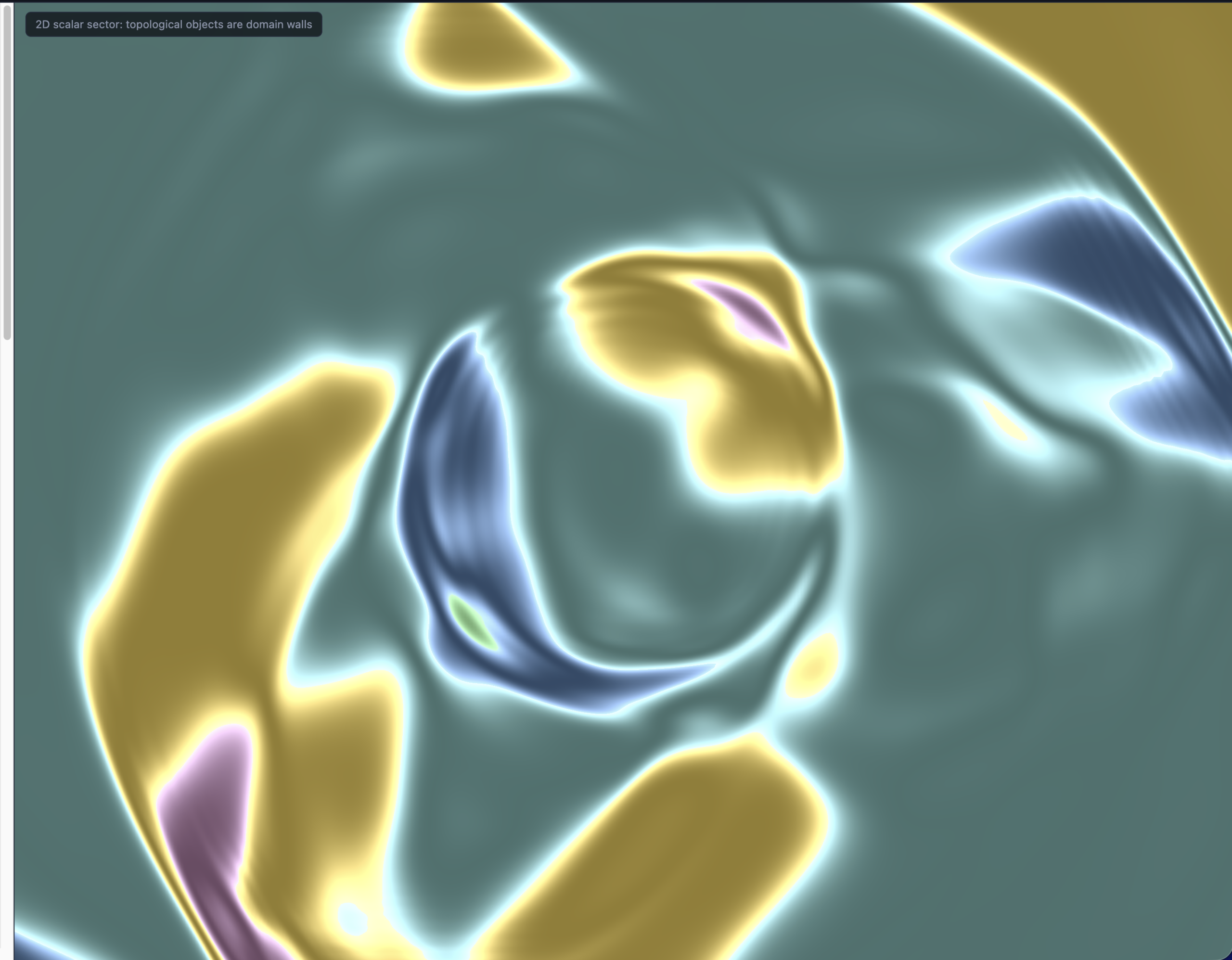
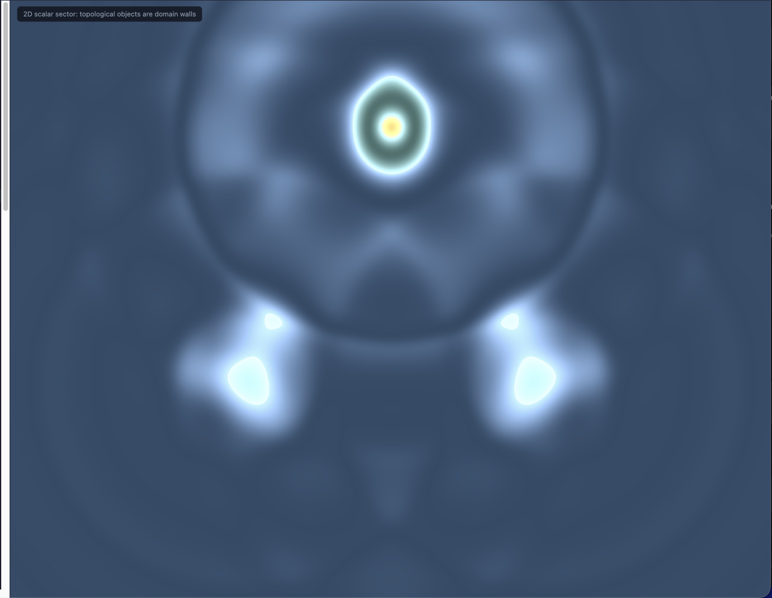
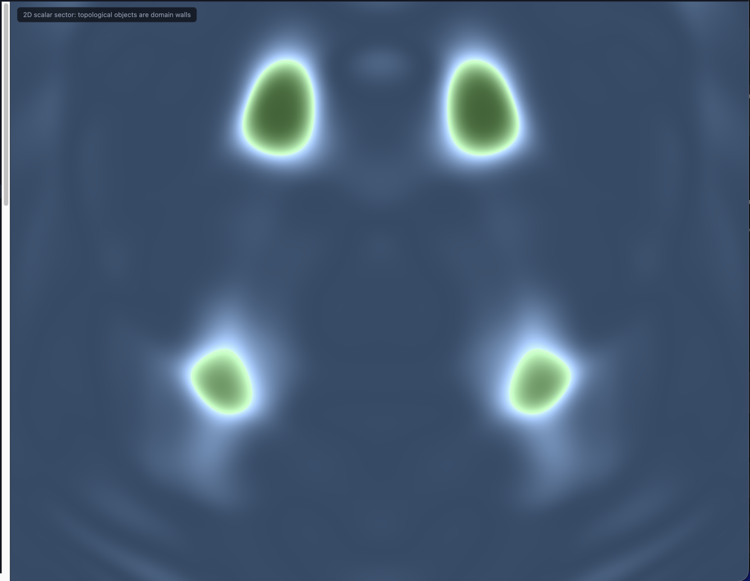
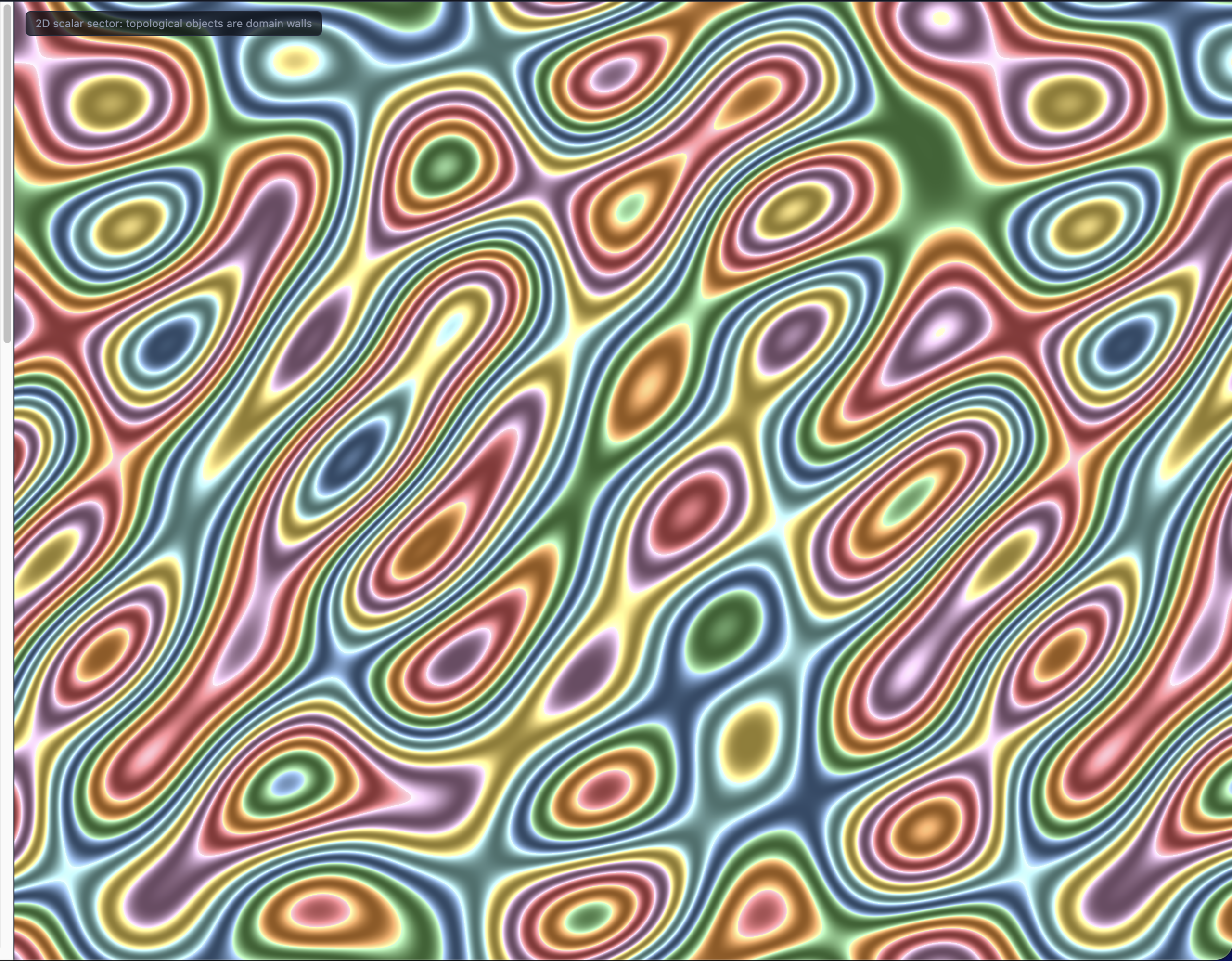
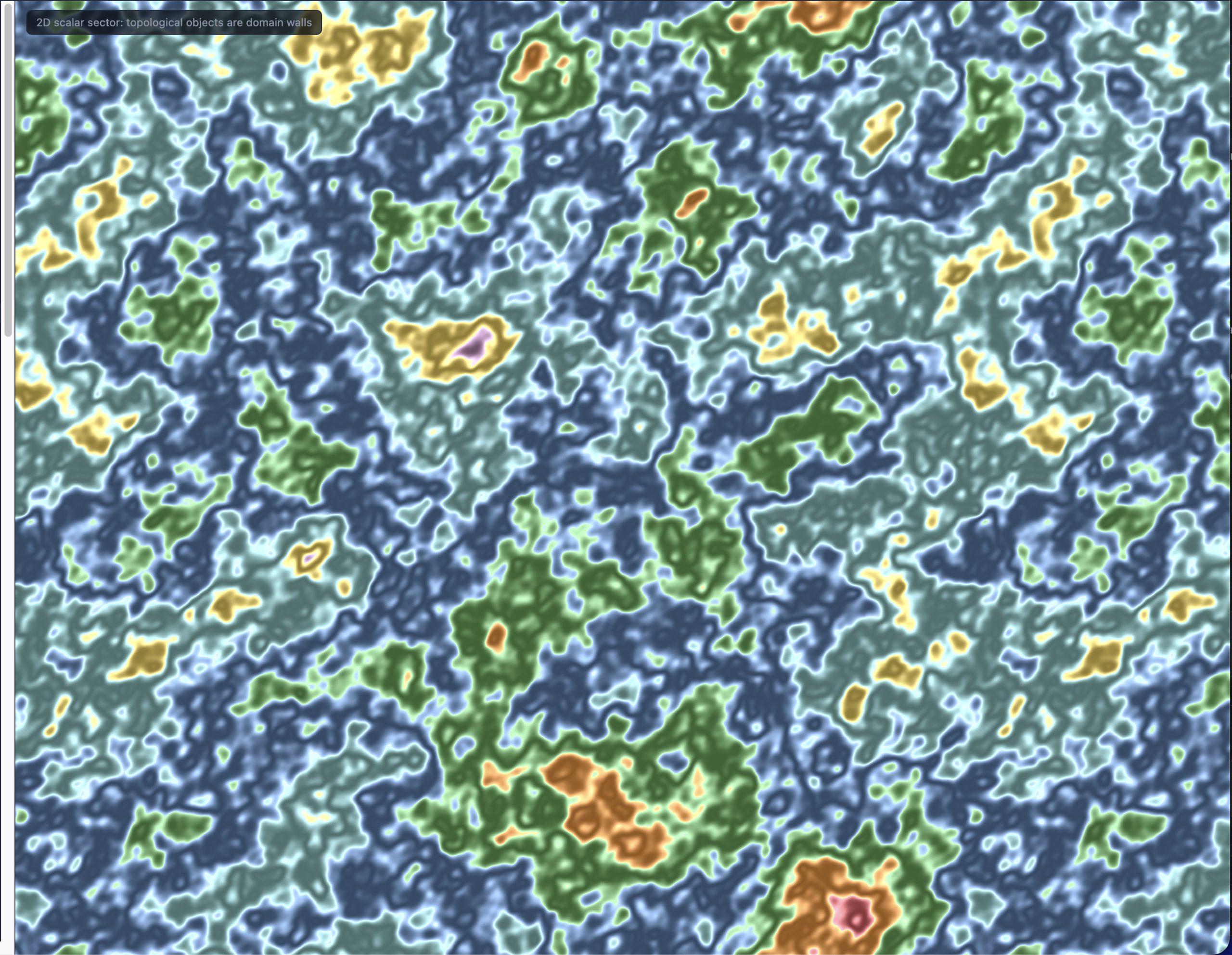
In two dimensions the same equation is integrated on a 512×512 periodic grid, on your GPU. Here the topological objects are not point-like kinks but domain walls — one-dimensional boundaries between regions sitting in different vacua — and the honest physics is that integrability is special to one spatial dimension. In 2D, curved walls have tension: they contract, merge, and straighten from geometry alone, in both Pure and Perturbed dynamics. Watching the “random” preset organize itself from a noisy mixture of all seven vacua into large coalescing domains is the best intuition-builder in the app.
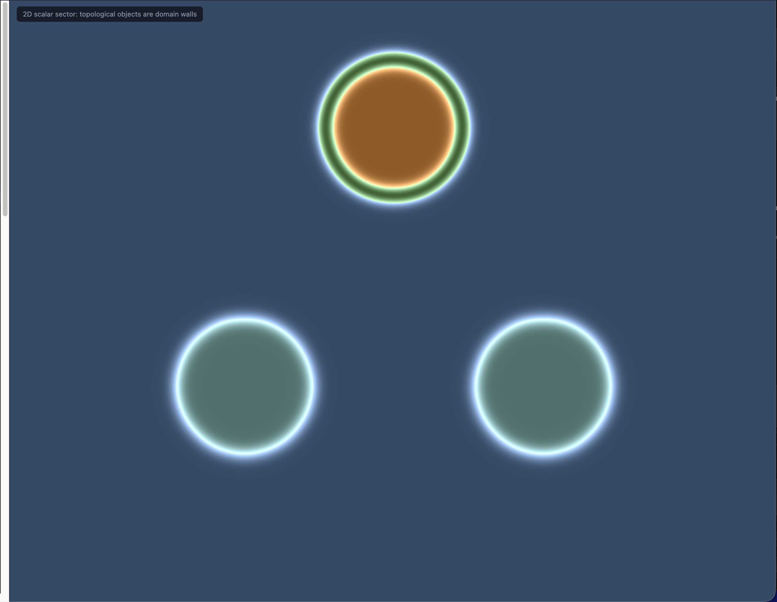
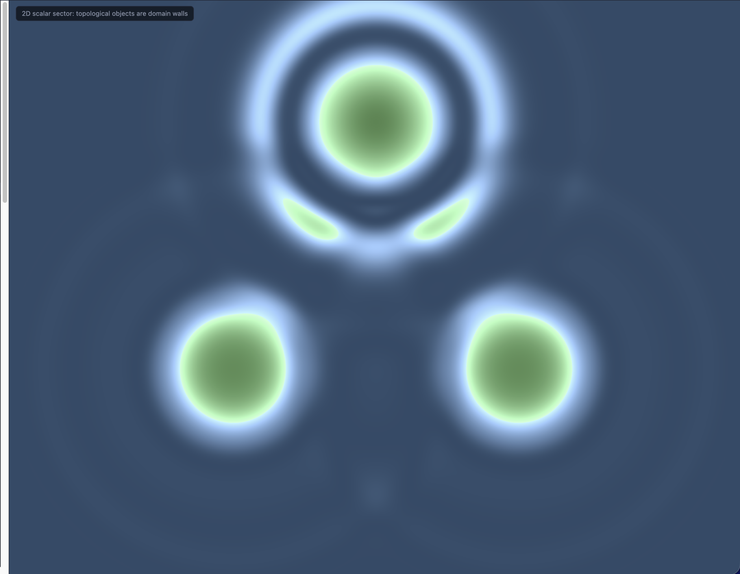
You can paint vacua by hand with a brush, or load presets, including a proton (two up-quark domains and one down-quark domain, uud, with charges +2/3 +2/3 −1/3 = +1) and a neutron (udd, summing to 0). These are labeled illustrative only, and the label is doing real work: this pure scalar field has no color/gauge sector, so nothing in the simulation actually confines the three quark-sector domains into a bound state. The app tells you to watch whether they stay clustered or drift apart — and the answer (they merge or drift; nothing binds them) is itself an honest demonstration of what a single scalar field does and does not contain.
The 2D mode also turns an expectation into a measurement. The no-go theorem implies an isolated winding-carrying domain has no topological protection in 2D — wall tension should shrink it steadily to nothing. The isolated-domain size vs. time panel tracks the area of an isolated bubble live, fits linear and exponential trends to the history, and reports the measured decay rate (or tells you honestly if the trend is statistically indistinguishable from flat). Seed the “single bubble” preset and you can empirically confirm a prediction of the theory in about a minute: a monotonic, roughly linear-in-time area collapse, with no anomalous stability plateau.
3D: what the theory actually says is there
The 3D mode is deliberately different, and its label is the most important one in the app: it is a static illustration, not a live 3D field simulation. It renders the certified extended structure from the no-go theorem — either a single flat domain wall separating the vacuum from a selectable particle sector, or three walls meeting along a shared axis (a “triple junction,” the 3D analogue of a 2D preset you can evolve live).
The reason this mode shows walls and junctions rather than floating blobs is the whole point of the section above: floating blobs are proven impossible. The accompanying “Why not a compact particle?” panel states the quantitative facts: the wall tension is about 23.5 GeV per square femtometer (the elementary kink mass per unit area), and the triple-junction line carries a real, exactly computed excess energy of 8 kink masses ≈ 2320.8 MeV — but neither rescues a finite-energy compact particle, because the wall sheets themselves still cost energy proportional to their unbounded area. The honest 3D picture of this field’s classical winding-carrying configurations is extended geometry, and that is exactly what gets drawn.
“What if the derived constant were different?”
My favorite small feature is a checkbox in the Advanced panel: “Explore: what if the SCC weren’t satisfied?” It exposes a slider for a hypothetical field mass parameter, defaulting to (and clearly marking) the derived value of 1776.86 MeV, with a live table of the consequences — kink mass, kink width — and an explicit numerical verdict comparing the hypothetical kink mass to the real 290.10 MeV.
There’s a nice piece of physics in how this works. The field equation in natural units contains no mass parameter at all — it is scale-covariant — so the slider never touches the running simulation. Only the conversions to femtometers, MeV, and seconds change, and they change live and exactly. The demonstration is the point: the dynamics you’re watching are universal, and the single dimensional number the theory derives is precisely what pins them to our universe’s scales. Nothing is tuned; there is nothing to tune.
How this fits the larger program
This visualization is a window into one chapter of a much larger structure. The GTE/UGP corpus currently spans 56 papers (P00–P55), covering the derivation chain from the self-containment axioms through the Standard Model’s gauge group, particle spectrum, and coupling constants, to quantum mechanics, gravity, and cosmology. A distinctive feature of the program is machine verification: the core results are formalized in Lean 4 — more than 400 modules in the canonical public repository, with zero sorry (no unproven placeholder steps) in the certified results — so the load-bearing claims are checked by a proof assistant rather than resting on my say-so. The corpus is careful to distinguish claim strengths throughout: machine-certified results, full analytic derivations, and computational confirmations are labeled as such, and the visualization inherits that discipline in its exact/proxy/illustrative labels.
Go deeper
- The live app: novaspivack.github.io/ugp-physics/visualizations/phimdl_kink_dynamics — runs entirely in your browser, no installation.
- Source code: github.com/novaspivack/ugp-physics (the app lives under
visualizations/phimdl_kink_dynamics/). - The complete theory (P48), The Complete GTE Framework: Standard Model, Gravity, Quantum Mechanics, and Cosmology from Φ_MDL — the monograph whose kink-dynamics chapter this app implements, including the no-go theorem and the Fock-space particle characterization: https://doi.org/10.5281/zenodo.20560550
- The Φ_MDL field paper (P42), The Φ_MDL Field: Quantum Structure, Born Rule, and Continuum Completion of the Chiral Minkowski CA — the field’s quantum structure in detail: https://doi.org/10.5281/zenodo.20417576
- The completeness paper (P43), The Complete Φ_MDL Framework: Algebraic Necessity, Quantum Mechanics, Emergent Gravity, and Uniqueness — why this field, and not some other object, is the substrate: https://doi.org/10.5281/zenodo.20417578
- The survey and reader’s guide (P00) — the recommended entry point to the corpus: https://doi.org/10.5281/zenodo.20168774
- The full corpus record (always resolves to the latest version): https://doi.org/10.5281/zenodo.20171558
- The Lean 4 formalization (canonical machine-verified library): https://doi.org/10.5281/zenodo.19574777
An overview of the whole physics program, with all papers and repositories, is on my research page: novaspivack.com/research/physics-program.
Open the app, load the pure-gas replay, and watch a few hundred collisions resolve without a single annihilation. Then flip on the perturbation and watch a slow pair spiral into radiation. That difference — and the fact that you can check both against exact solutions while they run — is what it looks like when a theory shows its work.