This is a browser-based cellular automaton in which two cooperating neural agents learn — in real time, from scratch — to keep the simulation alive and interesting. No pre-training, no external data. The neural network trains itself as the simulation runs, and the agents use what they’ve learned to steer the system away from death and toward sustained complex behavior. Companion experiment: for spatial parameter fields, beam-search lookahead, and greatest-hits snapshots, see Neural CA: Spatial Parameter Fields and Greatest-Hits Memory.
▶ Run the simulation in your browser ↗
(Works best on a modern desktop browser. Click Run / pause to start. The agents begin tuning after ~30 controller steps once the network has enough data.)
Gallery
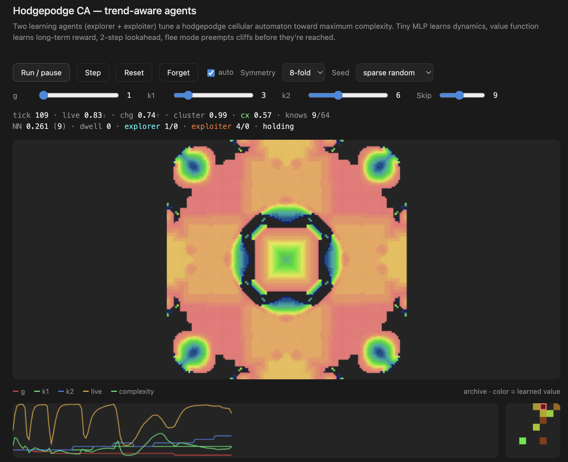
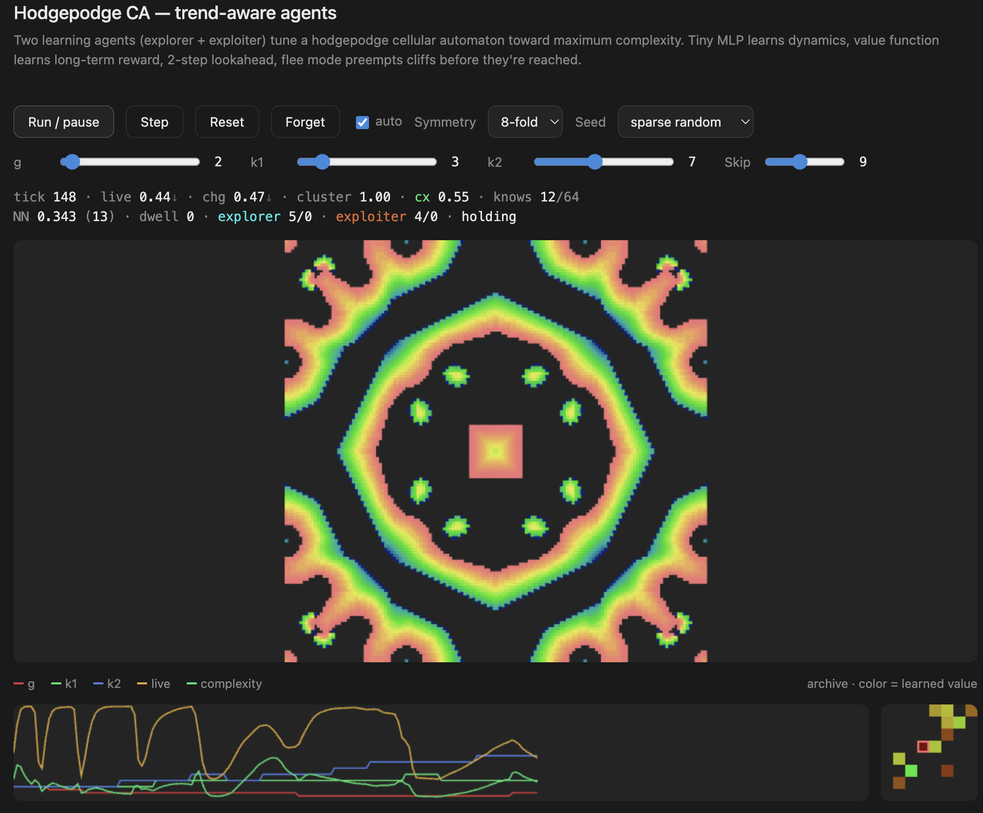
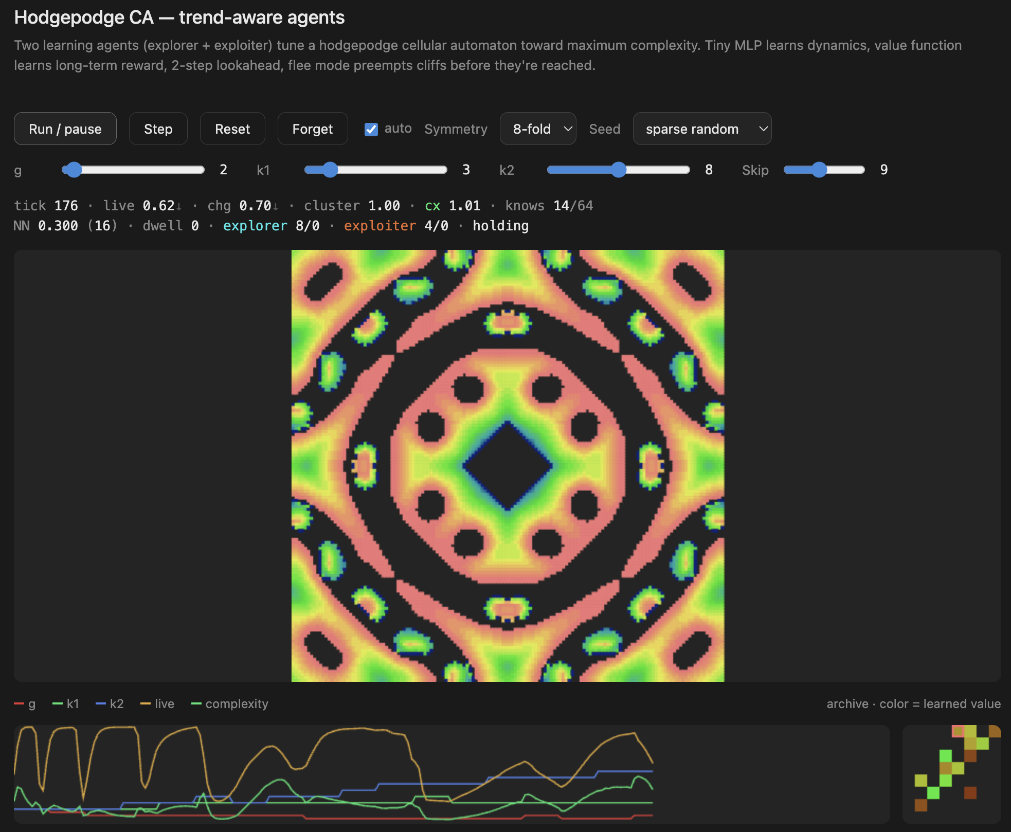

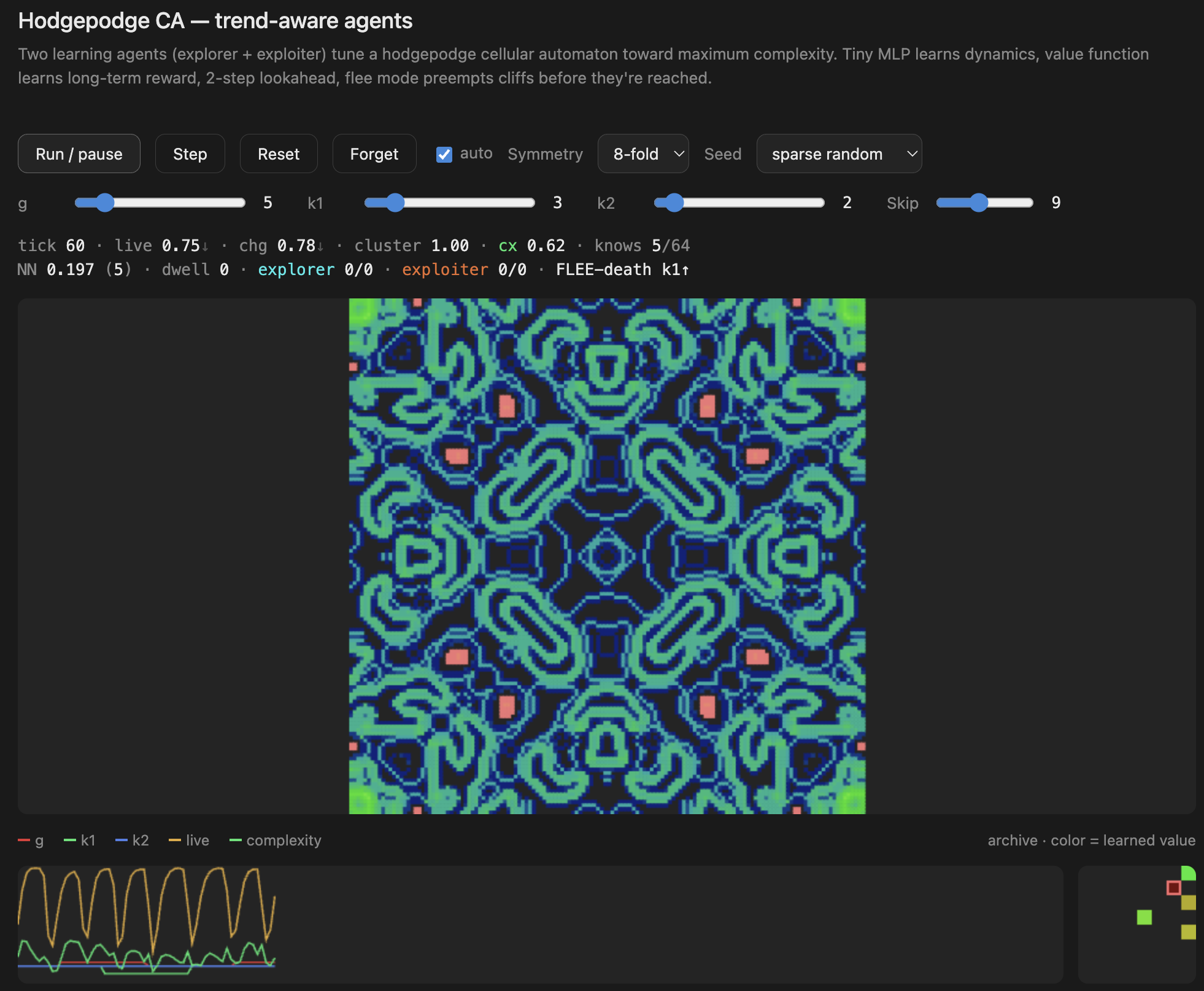

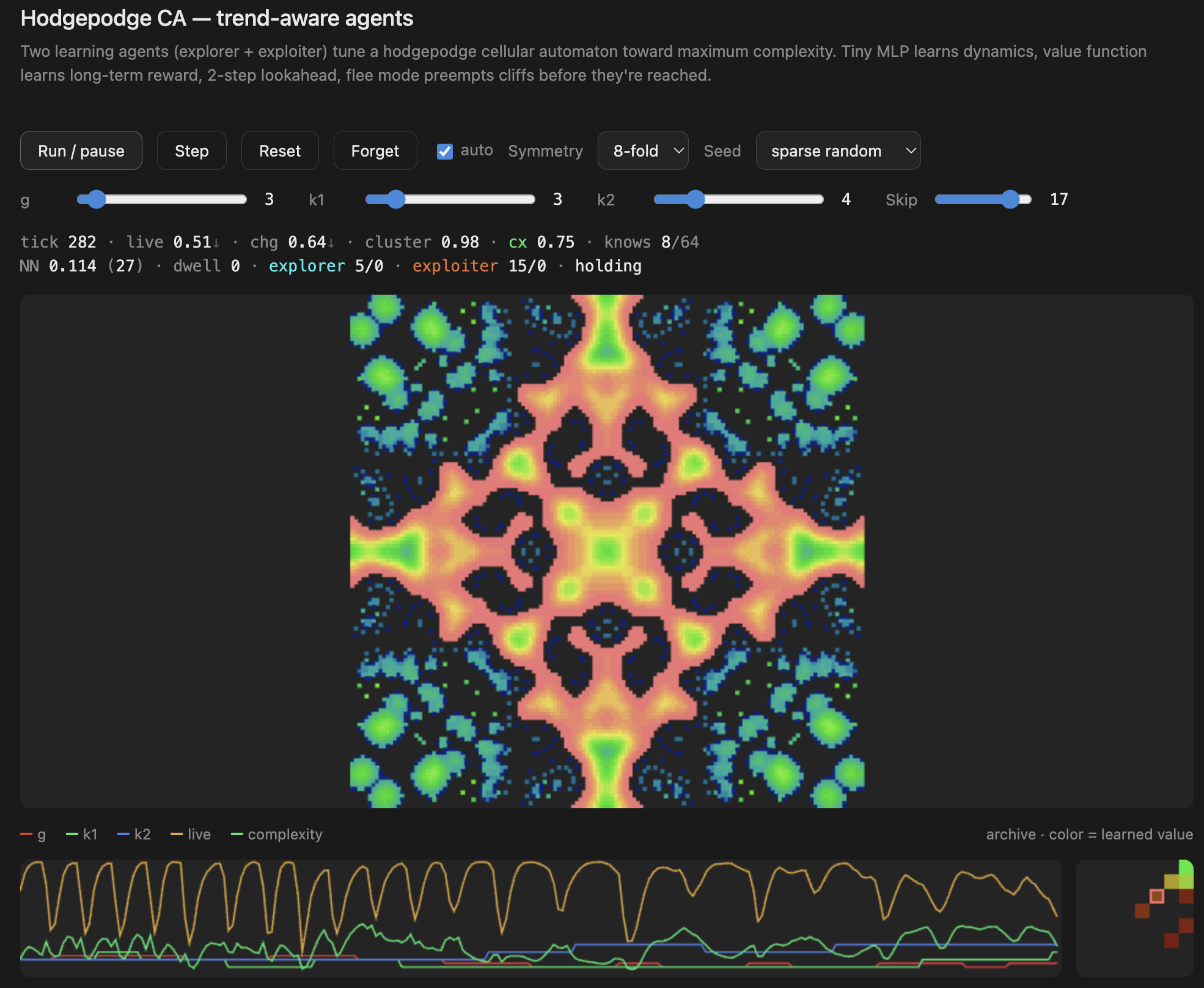
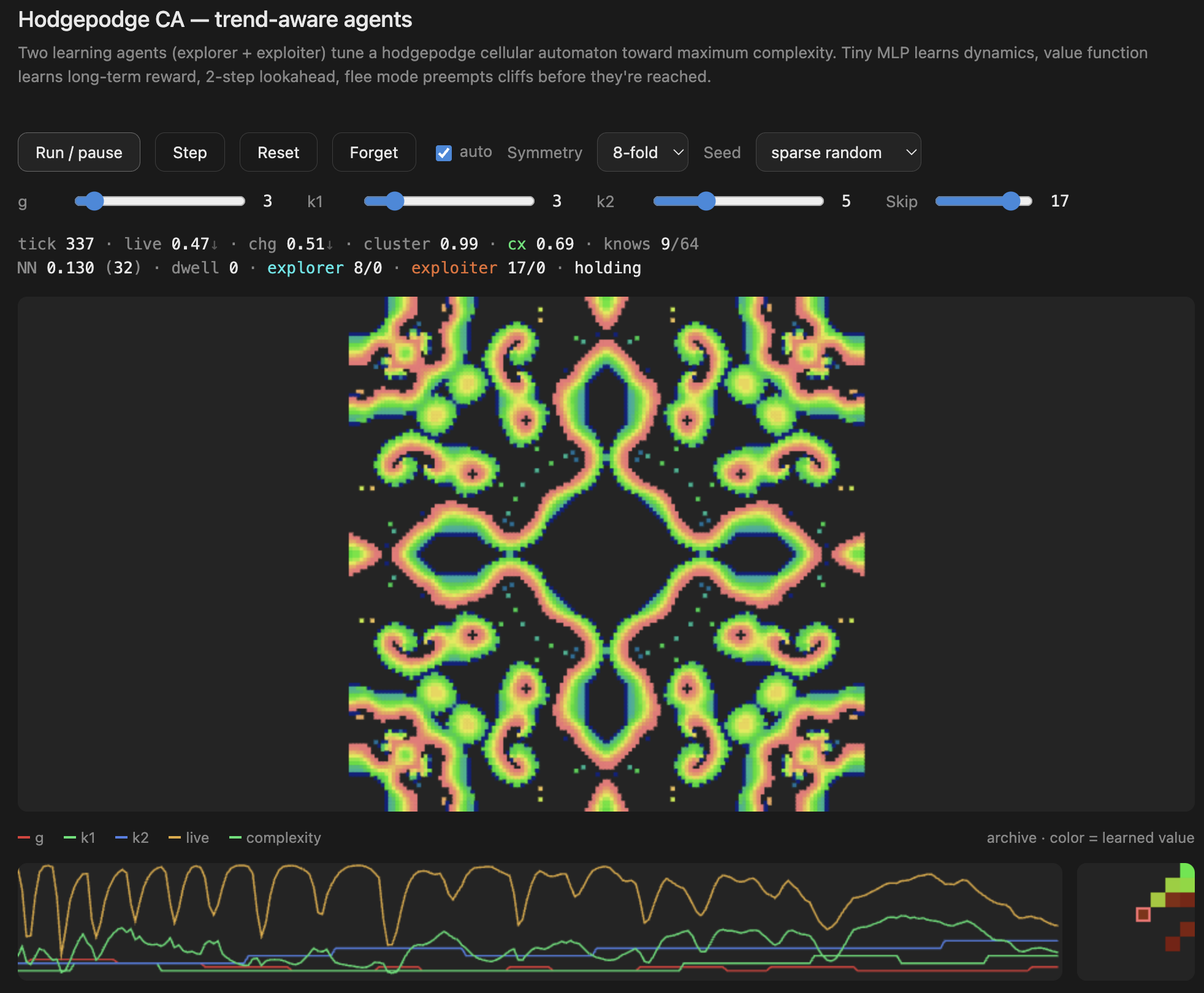
What this is
The underlying grid uses a hodgepodge-style cellular automaton — a reaction-diffusion rule with three states (healthy, infected, ill) and three parameters: g (growth rate), k1 (infection threshold from healthy neighbors), and k2 (infection threshold from ill neighbors). Different combinations of g, k1, k2 produce wildly different behaviors: static death, chaotic noise, frozen crystals, or — in a narrow band between — rich flowing structures.
The neural controller’s job is to find and stay in that narrow band. It does this by continuously adjusting g, k1, and k2 in small steps, guided by a learned model of how each change will affect the system.
How it works
The neural network
A tiny MLP (15 inputs → 16 hidden → 4 outputs) trains online using gradient descent. Its inputs are the current live-cell fraction, change rate, edge density, state variance, the current parameter values, a one-hot encoding of the proposed action, and two boredom signals (an instantaneous stability score and its smoothed average). Its outputs predict how each of those four statistics will change if that action is taken. After each controller step the network receives the actual outcome and trains on the error. No batches, no pre-training — it learns purely from experience as the simulation runs.
The value function
A tabular value function covers an 8×8 grid of (live fraction, change rate) bins — 64 possible behavioral states. Each bin stores an estimated long-term complexity reward, updated with temporal-difference learning (TD(0)) every controller step. This gives the agents a sense of which behavioral regimes are worth seeking out over time, not just immediately.
Two agents: explorer and exploiter
Two agents alternate control. The explorer weights novelty highly — it wants to visit behavioral bins it hasn’t seen before. The exploiter prefers to mine known high-complexity regions. Both use a 2-step lookahead: they simulate each candidate action through the learned model, then simulate one follow-up action, and pick the sequence with the best predicted outcome. This gives them limited foresight without expensive search.
Trend-aware flee mode
The key novelty in this experiment is preemptive control. Rather than reacting once the system has already died or frozen, the controller tracks short-term trends in live fraction, change rate, and complexity over the last 5 steps. If a trend indicates the system is heading toward a bad attractor — even if it hasn’t reached one yet — a flee mode fires immediately, overriding the normal agent logic and steering hard away from the cliff. This catches collapses before they become irreversible.
Interest, boredom, and long-run value
The agents maximize a composite complexity signal from live density, change rate, structure, and motion. A high score for a moment is not enough: if traces go flat and the pattern stops developing, the run can still feel stuck. The simulation computes a boredom measure from how stable live, change, and complexity have been over a recent window, weighted by how rich the activity looks. A smoothed boredom score is subtracted from the reward used to update the tabular value function, so bins that correspond to long, uneventful plateaus earn lower long-term value even when raw complexity looked fine. That nudges learning toward regimes that stay engaging over time.
Boredom also feeds into action selection and exploration: when it rises, the controller mildly favors novelty — visiting under-explored (live, change) regions — without swinging into constant chaos. The MLP sees the same signals, so predicted dynamics can account for a system that is drifting out of a dull attractor rather than twitching at random.
What to watch
- The status line shows the current controller action:
explorer g↑,FLEE-death k1↑,EXPLORE jump - The archive panel (bottom right) is the learned value function — watch it develop structure as the agents discover which behavioral regions are rich
- The trace panel (bottom left) shows the parameter history (g, k1, k2) and complexity over time — you can see the agents nudging parameters and the system responding
- The knows counter shows how many of the 64 behavioral bins the agents have visited
Code
Single self-contained HTML file, no dependencies. View source on GitHub ↗ · neural-ca repo ↗
Related post: Neural CA: Spatial Parameter Fields and Greatest-Hits Memory — same learning stance with spatial fields, beam search, and snapshot memory.